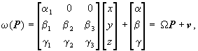
As we mentioned before,  by  s(D,M)we denote both the IFS and the  interpolation scheme (depending on M = {M_i, i = 1,.., n})  that associates to  D Ì R³ the  function  f whose graph F_D,M is the unique attractor of s(D,M).

 Definition 2. An  interpolation scheme s(D,M)  is invariant upon  transformation w: R³® R³  iff for any DÌ R³,

where F_D,M  denotes the attractor of the IFS s(D,M).

Definition 3. An  interpolation scheme s(D,M)  is  weakly  invariant upon  w  iff  there exists a set of matrices M' = {M_i', i = 1,.., n} such that, for any DÌ R³,
 

Note that invariance upon w is weak invariance with M' =M.

In this section we will examine the invariance of the interpolation scheme  introduced according to Theorem 1  with respect  to affine mappings w: R³® R³ having the same structure as transformations w_i, more precisely
 

                                    (14)

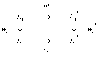
 with a, a₁,  b, b_i  and  g, g_i  real parameters, and  a₁ > 0. We will give conditions for the strict invariance of the general scheme, and will also discuss an interesting and very useful case of  weak  invariance.

Let  w transform the data set D into the set of points  w(D) = D^*= { P_i^* = [x_i^*  y_i^* z _i^*], i = 0, 1,..., n}. Notice that the special form of the matrix  W introduced in (14) guarantees that w transform pairs of points having strictly increasing abscissas into pairs of points having the same property, therefore it is possible to build  the IFS s(D^*,M ) = {R³; w₁^*, ..., w_n^*} and consider the  interpolation function corresponding to the transformed data set. At this point we need a general lemma,  first. Also let (f_° g)(x) = g(f(x)).

Lemma 2. Given the IFS s(D) = {R³; w₁, ..., w_n} and  a  transformation  w having equation (14),  if w_i° w  =  w_° w_i^*  (i = 1,..., n) ,  then

Proof. Let G denote the piecewise linear interpolant of D. Then the   Hutchinson orbit of G is a sequence of polygonal lines  converging (in Hausdorff  metric) to F_D, let this be {L_k = W ^k(G), k = 0, 1,...}. Also denote by  L₀^* = w(L₀)  the piecewise linear interpolant of  D^* = w(D), and let L_k^* = W^*(L_k-1^*), k = 1, 2,... where W^*( . ) = È_i w_i^*( . ). The sequence {L_k^*} is the Hutchinson orbit of w(L₀) and, therefore, F_w(D) = lim_{k ®¥} L_k^* . If the diagram
 

                                                  (15)

commutes for all i, namely  if  w_i° w = w_° w_i^* , then at  every new iteration k it holds  L_k^* = w(L_k), which means that F_w(D) = lim_k®¥ L_k^*  = lim_{k ®¥} w(L_k) = w(F_D) , being w a continuous function in R³.  à

Lemma 3 (Translation case).  Let  the affine mapping  w be the  translation  w(P) = P + v,  or,  equivalently, let W = I  in (14). Then the interpolation scheme is strictly invariant under  w, namely (12) holds.

Proof. According to (5)  w_i (P) = P_i +A_i (P -P_n) and, analogously w_i^*(P) = P_i^*+A_i ^*(P -P_n^*),  with
 

                                                     (16)

Then  w(w_i (P)) = P_i + A_i (P-P_n) + v  and  w_i^* (w(P)) = P_i +  v + A_i^*(P -P_n). Therefore, for any arbitrary point P Î R³ we have d_i(P)= w_i^*(w(P)) - w(w_i (P)) = (w_°w_i^*-w_i° w)(P) = (A_i^* - A_i)(P -P_n), and therefore  d_i(P)= 0  if and only if  the matrix   D  = A_i^*- A_i = [d_jk] is the zero matrix. Direct computation shows that for M=M', d_j2 = d_j3 = 0,  j = 1,2,3,  while  d₁₁ =  a_i^*-a_i = 0,  d₂₁ =  c_i^*-c_i = 0,   d₃₁ = k_i^*-k_i = 0 . So,  d_i(P) = 0, i.e., the diagram (15) commutes.  à

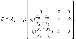
Lemma 4 (Linear case). Let  the affine mapping  w  have zero translation part, v = 0, so that it reduces to the linear transformation  w(P) =WP.  Let  W have lower-triangular form with g₂= 0. Then,  (12) is valid if and only if  b₂ = g₃.

Proof.  Under the assumptions of the Lemma, the difference d_i  will have the value d_i = (w_°w_i^*- w_i° w)(P) = (A_i^*W - WA_i)(P -P_n), where A_i^* is given by (16). For M=M', the matrix D = A_i^*W -  WA_i has the following form

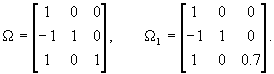
So, D  is the zero matrix for all feasible M if and only if  b₂ = g₃. Then, d_i= 0, the diagram (15) commute, and w(F_D,M) = F_w(D),M. à

The Lemmas 2, 3 and 4 can be combined into

Theorem 3.  Let the affine mapping  w be defined by (14). Let the matrix W have  lower-triangular form with g₂= 0. Then, the interpolation scheme s(D,M)is strictly invariant under  w, namely (12) holds if and only if  b₂ = g₃.

The next example uses a specific visual approach to illustrate Theorem 3.

 Example 3.  Let D = {(0, 0, 0), (1/4, 0, 1/2), (1/2, 1/2, 1/2), (3/4, 1, 1/2), (1, 1, 0)}be the data,  and let the choice d₁= 0,  d₂= 1/4,  d₃= 1/4, d₄= 0,  h₁= 0, h₂= 0, h₃= 0, h₄= -1/4, l₁= 1/4 , l₂= 0, l₃=l₄=-1/4, m₁= 0, m₂= -1/4, m₃= 1/4, m₄= 0 be made. By this, the parameter matrix set M is fully determined as well as the hyperbolic IFS s(D) ={R³; w₁, w₂, w₃, w₄}with the attractor F_D. Further, consider two different linear maps w(P) =WP and q(P) =W₁P, where W  and W₁ are defined by

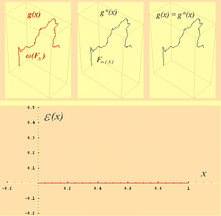
The Figure 4 (above) shows three diagrams.  The leftmost one is the graph w(F_D), the middle one is F_w(D) and the rightmost one represents  both graphs simultaneously. Let the vector valued function g(x), 0 £ x £ 1, correspond to the graph w(F_D) and let g^*(x), 0 £ x £ 1, correspond to F_w(D). To compare two graphs better, the function e(x) = |g(x) -g^*(x)|, 0 £ x £ 1, is calculated (Fig. 4, below).

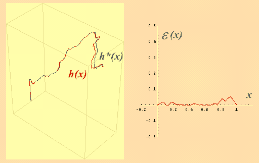
 Let q(F_D) be the graph of the function h(x),  0 £ x £ 1, and let F_q(D) be the graph of  h^*(x),   0 £ x £ 1. The Figure 5 shows the similar comparison as above. This time the difference between the  graphs q(F_D) and F_q(D) (or h and h^*) is visible (left). This is proved by the graph of e (x) = |h(x) - h^*(x) |, 0 £ x £ 1, being different from zero.

The following theorem gives the conditions of weak invariance of an interpolating IFS.

Theorem 4. Let s(D,M)be a hyperbolic block diagonal IFS. Let  w be defined by (14) with W being a regular block diagonal matrix (  b₁ = g₁= 0 ).Then,  the scheme  s(D,M) is weakly invariant under  w, namely (13)  holds.

Proof. Since s(D,M) is a block diagonal, there exists a hyperbolic IFS t(D_yz,M) so that s(D,M) is its lifting (Definition 1), i.e., the 2D data set  D_yz = {Q_i = [ y_i  z_i]^T , i = 0, 1,..., n} obey conditions (11). In the matrix form, these conditions are
 

where r_i = [ f_i   g_i]^T .  Since the scheme s(D,M) is invariant upon translation (Lemma 3), one can restrict transformation w given by (14) to the linear case w(P) = WP with W being a regular block diagonal matrix

Now, w(P_i) = [a₁x_i b₂y_i+ b₃z_i g₂y_i+ g₃z_i]^T or, shortly w(P_i) = [a₁x_i (NQ_i)^T ]^T. Multiplying (17) with N from the left, and using I = N^-1N  (since W is regular, N  is invertable) one gets

which, by denoting

Equations (19) are conditions (11) for the data set D_yz^* with v_i^*(y, z)  = M_i^*[y   z]^T + r_i^*. Since M_i^*and M_i are similar matrices, they share eigenvalues, so t(D_yz^*,M') is also a hyperbolic IFS and M' = {M_i^*, i = 1,.., n}. Let D^* be a lifting of the data D_yz^* on the mesh  x₀< x₁< ...< x_n and  let s(D^*,M') be the lifting of t(D_yz^*,M'). By Theorem 2, s(D^*,M') = {R³; w₁^*, ..., w_n^*} is also a hyperbolic block diagonal IFS.  Let M_i^* be the lower-right 2x2 block of the matrix A_i^* that corresponds to the mapping w_i^*. Then, the first equality in (18) implies  A_i^*= WA_iW^-1 or A_i^*W = WA_i, for i = 1,..., n, i.e., by Lemma 2,  w( F_D,M) = F_w(D),M' .